Categories
Results

Alpha Drop

Hedge fund week just wrapped up here in Miami, and I had the chance to catch up with some industry friends like fellow Croatian and former podcast guest Vuk Vukovic. A big shoutout to Vuk and the incredible success of Oraclum Capital, his NYC-based hedge fund! Beyond motivation, these conversations always get us thinking—about how far we’ve come, the lessons learned, and the market patterns emerging. So, today, we’re switching things up a bit.

Breaking Down Thinking vs. Acting in Real-Time

These newsletters often dive deeply into trade theory—how to form opinions, identify dislocations, and structure trades to take advantage of them. Thinking critically about market context is just as important, if not more so, than taking action, as outlined in the case study linked here. But let’s be honest: we don’t always have the luxury of testing every idea before committing capital. Sometimes, decisions must be made on the spot, and more often than not, they’re more straightforward than they appear—they have to be.

To illustrate this, I share a slightly refined diary entry from a year ago, offering reflection and motivation. Market highs, uncertainty, and the fear of missing out create a lot of noise—but they also spark new ways of thinking. I hope this record and perspective spark new ideas on when and how to engage in markets this year ahead.

Take your time, enjoy the read, and try to focus on the bigger picture rather than getting lost in the details. Stay tuned for upcoming podcasts, explainers, and part two of the Market Tremors newsletter. Cheers, and let’s make some money.


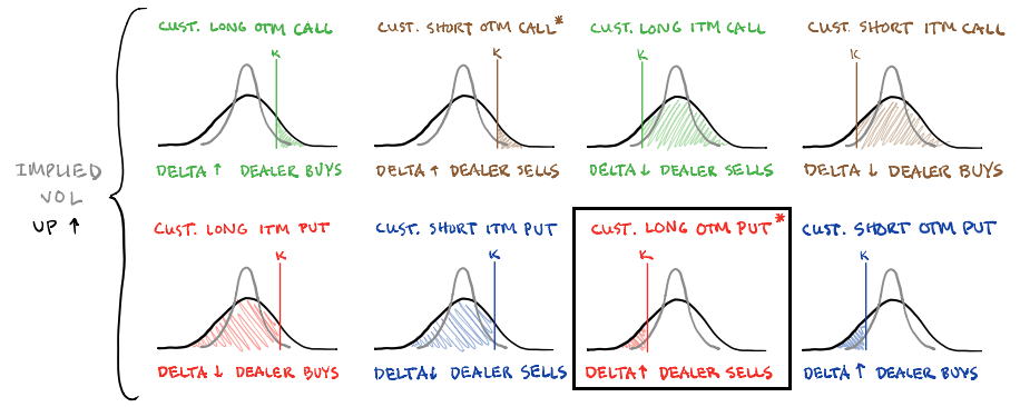
On February 16, 2024, my trading partner Justin pointed out a rich, elevated call skew in Super Micro Computer Inc. (NASDAQ: SMCI). This occurs when out-of-the-money call options carry higher implied volatility than at-the-money or in-the-money options, often signaling strong demand for upside exposure. At that point, SMCI had been climbing steadily for weeks, with the charts suggesting a parabolic advance and an imminent climax.

I spotted 200-wide 1×2 ratio spreads that could be opened for credit. Simply put, a ratio spread is an options structure in which you buy a contract at one strike and sell two (or more) at another, further away. I often use such a structure when volatility is more steeply skewed, meaning certain strikes—like deep out-of-the-money (OTM) calls—have much higher implied volatility (IV) because traders expect more risk or extreme moves in that direction.

IV is the amount of movement traders anticipate. A higher IV means the market expects more significant price swings, leading to more expensive options, while a lower IV suggests less expected movement, making options cheaper—factors like earnings reports, economic data, or overall market uncertainty influence IV.

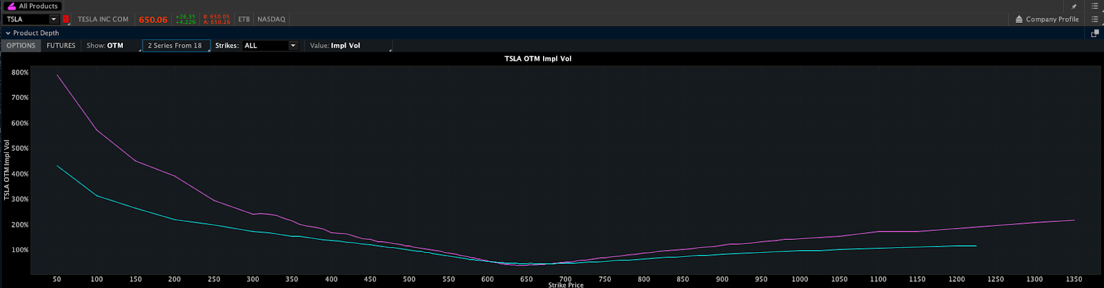
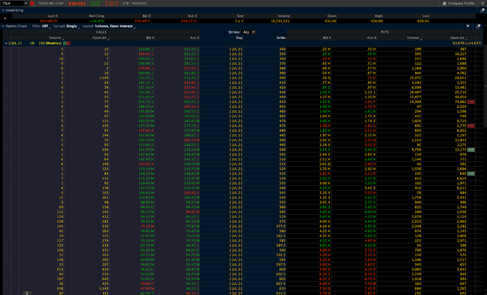
In this case, using Schwab’s thinkorswim lookback feature, implied volatility on the call side ranged from the mid-100s near the current market price to over 200% at the furthest strike. On the put side, things got even wilder—volatility climbed from the mid-100s near the market price to several hundred percent at the farthest strike, as pictured below. When volatility is this high in far-out-of-the-money options, traders are piling in—either looking for protection or betting on a big, unexpected move.

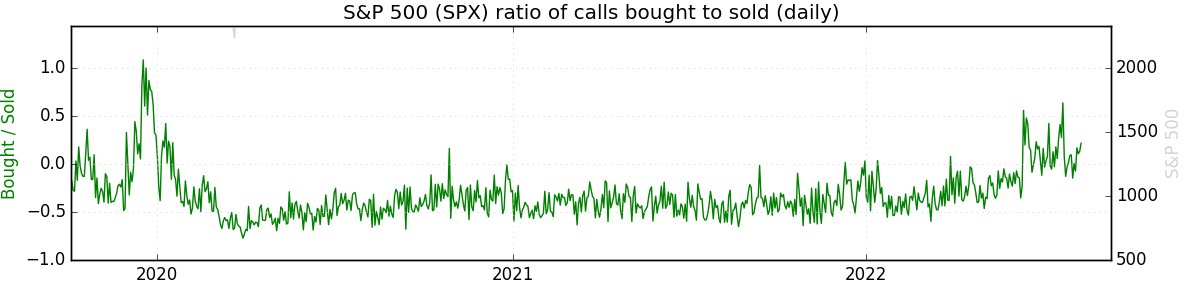
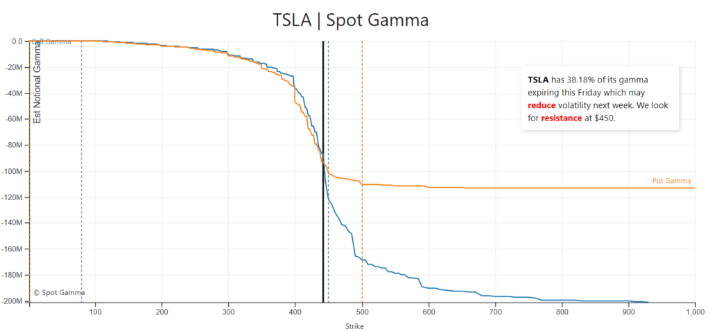
As the stock was pulled back from its highs, we observed that the excitement in call-side volatility had begun to diminish—it wasn’t as intense as it had been a month earlier, according to SpotGamma data. This served as a key signal for us. A declining enthusiasm for calls indicates that traders are less inclined to chase the stock higher. We were prepared to act on this shift, betting that the stock had reached an interim peak; this was great news for us, as our options structures tend to perform best when volatility stabilizes and the stock drifts rather than making significant, protracted moves.

Right after the market opened, the 23 FEB 24 1300/1500 spread flipped from a 0.50 debit to over a 1.00 credit to open. I didn’t catch it right at the start, but about an hour later, I spotted the opportunity. The pricing looked solid—it offered a credit to close at the money—and everything checked out risk-wise according to my rules. So, I decided to dip my toes in with five units, keeping it on the smaller side for this trade. This all went down on February 16.

SOLD -1 1/2 BACKRATIO SMCI 100 (Weeklys) 23 FEB 24 1300/1500 CALL @1.10

All else equal, if the trade were entirely in the money (ITM), meaning the short strikes are right around the current market price, it would price for about 40.00 credit to close. At the money (ATM), right around the current market price, the structures traded for around 12.00 credit to close. This quick check suggests we’re good to move forward. Here are the orders for one account. You can find a summary screenshot of all orders at the end of this letter.

Given the risk involved in this trade, the abovementioned account could take on a maximum of 8 units. As we’ll see later in this entry, I pushed those limits, possibly going beyond what’s typical for me. However, I justified this by considering the distance between the stock price and the strikes used in the trades, which felt like a safe cushion to work with.

$320,000 (Net Liquidation Value) / $38,000 (Daily Loss at +1 EPR if the Spread’s Long Strike is ATM) = 8.4 units. EPR represents the brokerage firm’s estimate of the maximum expected one-day price range for an underlying security. Net Liquidation Value refers to the total value of a portfolio if all positions were liquidated at current market prices. Here are more details.

A few hours later, implied volatility dropped across the board, with the further out-of-the-money (OTM) options seeing the most significant decline. The implied volatility of the options closest to the stock price fell moderately, while the farther OTM strikes experienced a more substantial drop. This shift worked in our favor and helped make the trade profitable.

The long strike I owned (1300) had an implied volatility of ~190% before, which dropped to ~165% after.

The short strike I sold (1500) had an implied volatility of ~215% before, which dropped to ~180% after.

The trades were closed on the consolidation following the sharp morning liquidation. Here are the trade tickets.

BOT +1 1/2 BACKRATIO SMCI 100 (Weeklys) 23 FEB 24 1300/1500 CALL @-1.05

From the panicked price movement, it looked like people late to the party were just selling off existing positions, not necessarily big new sellers entering the market; the stock might eventually retest those higher levels again. Even with the drop, implied volatility stayed high, which is crucial because it suggests continued uncertainty and anticipation of significant movement.

Given how sharp the sell-off was and how many traders were probably surprised by it, I decided to jump back into the trade on February 20—this time with a bigger position, especially after the long weekend when the market had some time to settle. Strikes and trade tickets follow.

SOLD -1 1/2 BACKRATIO SMCI 100 (Weeklys) 1 MAR 24 1300/1500 CALL @1.10

SOLD -1 1/2 BACKRATIO SMCI 100 (Weeklys) 1 MAR 24 1400/1600 CALL @1.10

SOLD -1 1/2 BACKRATIO SMCI 100 (Weeklys) 1 MAR 24 1350/1550 CALL @1.05

With the liquidation, the trade above was farther away from current prices than the last. Additionally, we moved it to next week’s expiry after the long weekend since it was no longer present for the 23 FEB 24 expiry. The lookback feature on Schwab’s thinkorswim shows implied volatility at the 1300 strike was ~180%, while at the short strikes, it was ~200%.

A quick check of SpotGamma’s implied volatility skew tool reveals a still-elevated call skew. Awesome!

Soon after, despite minor volatility shifts, we added similar trades with strikes that were further from the current price.

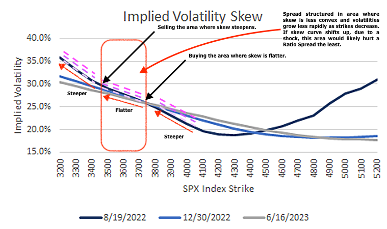
Gauging implied volatility accurately using the lookback feature can be tricky, but we observed that the difference in implied volatility between the strikes was narrowing. This indicated that the volatility skew was “flattening.” In simpler terms, the implied volatility between different strikes was becoming more similar, unlike a steeper skew where the farther strikes have much higher implied volatility. This can be good for the trade.

Here’s a chart that illustrates this “flattening” volatility skew. While this example shows the S&P 500, the concept is the same. Pay attention to the blue versus green line!

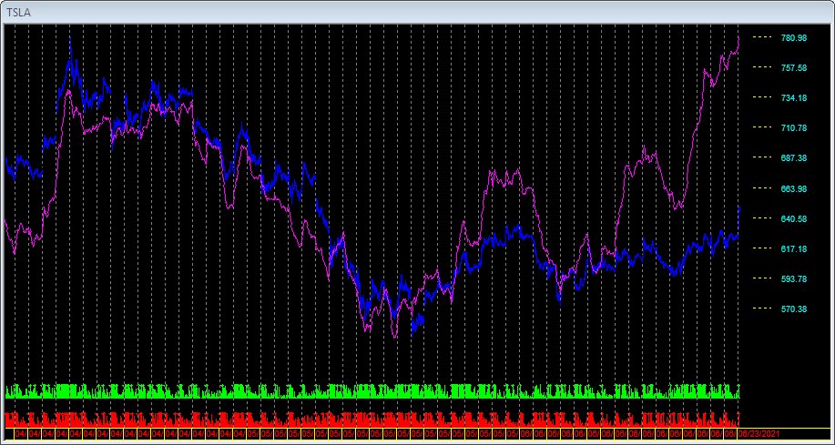
Anyways, back to the charts. So, here’s the price action. Straight down!

On February 22, we rotated more into similar structures we started working on February 20.

SOLD -1 1/2 BACKRATIO SMCI 100 (Weeklys) 8 MAR 24 1400/1600 CALL @1.10

At the time of entry, lookback showed the implied volatility of the 8 MAR 24 spreads was around 145% for the long and 155% for the short strikes. At the second entry, the volatility spread between the strikes started narrowing. Overall volatility came down, but the difference between the strikes was about the same.

Here’s what the volatility skew looked like at this point. This is a 30-day look back (the shadow).

I ended up closing the 1 MAR 24 spreads on February 22 for up to a 1.00 cr.

BOT +1 1/2 BACKRATIO SMCI 100 (Weeklys) 1 MAR 24 1350/1550 CALL @-.50

Here’s the implied volatility for the 1 MAR 24 options chain. Again, while a bit lower than when we started, the difference between the two is roughly the same. The passage of time is definitely working in our favor, here!

I’ll note that I closed prematurely because underlying price action suggested we could trend higher, with the upper VWAP band as an upside target. The spreads ended up pricing for $1.00 more in credit. Take what you can get, Renato!

The challenge we faced was deciding whether closing and rotating the trade early would lead to additional profits. Ultimately, we rolled the position and made money either way, but this was the thought at the time. In other words, are we doing too much?

After closing the 1 MAR structure, we added 8 MAR structures on February 22. Trade tickets for one account below. These additions made the position larger than I wanted, so I bought cheaper crash options to manage the margin (the amount of money required to maintain the position) first and foremost. It was a tense moment! Thankfully, with these additions, we stayed within our limits and didn’t breach any safety thresholds.

SOLD -12 1/2 BACKRATIO SMCI 100 (Weeklys) 8 MAR 24 1400/1600 CALL @1.05

BOT +3 SMCI 100 (Weeklys) 23 FEB 24 1580 CALL @.13

At this point, the lookback showed implied volatility for the short strikes was around 160%, while the long strikes were at 150%. The difference between the two was around 10%.

Again, IV refers to the market’s expectations of future price movement expressed as a percentage. A higher IV suggests more movement, while a lower IV suggests less movement.

This is what the chart looked like at that time.

Around 2 PM, the market struggled but recovered, finishing higher by the close. The trades moved against me slightly, but the ATM and ITM entry and holding criteria (i.e., credit to close) mentioned above were still met, so I stuck with it.

Regarding having to hedge, I just focused on the spread’s sensitivity to price movements. Despite intense price action, the Greeks were okay. I remained in the position for about a week and a half. After the first week, the spread moved in my favor, but not to the extent I had hoped.

To explain, implied volatility remained higher on the short strike but dropped more on the long strike. Had the volatility on the short strikes dropped significantly more, the spreads would have likely come off sooner. Pricing the 15 MAR 24 spreads, those were trading for a debit to close, and it did not make sense to do anything other than sit on my hands and wait. If the stock continued to rise, which eventually occurred, the spread had more potential. Here’s the lookback at the time.

This is the price chart at month-end. It felt like there was more room to go up.

After the weekend, there was a big overnight move. Traders caught the news that SMCI would be included in the S&P 500.

I used the gap as a gift and sold into it, monetizing spreads from 3.00 to 5.05 cr to close. Trade tickets for one account follow.

BOT +1 1/2 BACKRATIO SMCI 100 (Weeklys) 8 MAR 24 1400/1600 CALL @-5.05

5.05 marked the top in the structure’s pricing despite the stock moving higher after 10:00 AM. It took me years of watching these structures to spot softening sensitivity in the spread, prompting such closure. Had this gap not happened, the spreads likely would have been closed for small credits (0.05 cr). Again, the gap was a gift. Take it, Renato!

At this point, I am already considering rinsing and repeating this trade. The 15 MAR 24 200-point spread fully ITM traded for a small credit to close, which was unsafe. I widened accordingly to a 250-wide spread, priced for a very thick credit to close—the lookback shows about 44.00 cr. Here’s the lookback.

So, we went out to 1300/1550. There, I saw 1x2s pricing for thick credits to open.

SOLD -1 1/2 BACKRATIO SMCI 100 15 MAR 24 1350/1600 CALL @3.05

The implied volatility at the 1300 strike was ~150%, and at the 1550 strike, it was ~175%. We entered an hour early without regard for the stock chart (above), which was a costly mistake. The stock ripped higher, resulting in a ~$2.00 loss per spread.

Notably, the implied volatility skew steepened on the day of entry. Here’s a visual.

However, later that day, the spreads settled down. At 1:40 PM, the stock peaked, and the pricing of the 1300/1550 we put on declined slightly. To manage risk, I closed some units there. In any case, the spread narrowed, owing to a flattening and stickiness of the skew; 1300/1550 = 150/175% (~25% spread) → 140/160% (~20% spread). If I waited longer, the additional units would have gone massively in my favor. Oh, well!

Over the next few days, the stock moved down and then up; overall, the stock stayed flat. During this time, the spread increased in value, working in my favor. With these spreads, you want drift, not protracted movement!

My targets were at 5.00 and 10.00 cr to close, as I got over the next day or so. Implied volatility didn’t budge much. Based on thinkorswim’s lookback feature, it rose in the long strike more than the short strikes, which is what you want to see. Decay helped!

I wanted to hold longer because the spread 50 points closer to the money was pricing at 10.00 cr to close, about 3-5.00 cr more than I had my pricing for. Based on the stock price chart, we were peaking, but these moves tend to go sideways or higher for a bit longer. Candle shadows tend to get tested!

If we fast forward, the session was quiet, with SMCI trading sideways to lower from the open. The pricing of the spread went as high as 10.00 cr (at which point I started to monetize).

BOT +1 1/2 BACKRATIO SMCI 100 15 MAR 24 1350/1600 CALL @-10.05

Here’s what implied volatility looked like (i.e., a rise in the long strike, whereas the short strike stayed about the same).

After the close, I started thinking, “Man, I should have closed that last spread.” It went to my target, but I kept holding (correctly), as you want to maintain some runners. However, the price action was weak into the evening, after the market closed, and I was now concerned I would lose all or most of the profit in my remaining spread. Mental games, here. Patience, Renato!

The market opened sideways the next day. I monetized my last spread for 11.00 cr, close to its peak.

BOT +1 1/2 BACKRATIO SMCI 100 15 MAR 24 1350/1600 CALL @-11.07

Here are the implied volatilities at the exit (i.e., noticing the more significant drops in short strikes relative to the long ones).

There’s a critical factor that helped the trade keep its value. The stock went sideways, and a day or so passed, allowing some of the decay to kick in. The decay disproportionately affected the further OTM strikes (i.e., there’s more to decay than usual), with the lookback showing implied volatility dropped to 135% long / 150% short a few minutes after I closed my position. The market was attempting to go higher, volume was low on the 1300 strike, and the spread ended up pricing higher than what I closed it for. Bummer! Here’s what it looked like.

SELL -1 1/2 BACKRATIO SMCI 100 15 MAR 24 1300/1550 CALL @-15.70 LMT

On March 8, the market peaked, hitting the 1200 figure I had envisioned. 1200 was a target for me due to the amount of interest (open interest and volume) at that strike, as well as the trend of the market. The March 4 shadow would also be taken based on the March 5-7 price action. Essentially, we traded up to and held short of the March 4 high, and the spread increased in value by $10.00 cr. I could have doubled my profits for the trade, but at the risk of losing it if things had gone the other way. Remember February 22, when the extreme volume was at the 1000 strike and above? We failed there. This was a blow to options buyers!

On March 8, 10-15 minutes after the market opened, implied volatility for 1300/1550 per thinkorswim’s lookback showed a much more significant drop in further OTM strike as the stock went up by $33 in that one day. Vol down, stock up, weekend decay, and that’s how a spread that priced 5.00 cr to close two days before ended up trading to 25.00 cr to close. Here’s the lookback.

On March 11, the stock traded much weaker. Implied volatility on the 1300/1550 went to 150/170%. Despite this, the trade lost a lot of delta, which the implied volatility bump couldn’t make up. The lookback shows the trade went to a 7.00 cr, a ~70% loss. This is what I say you’re up against. There’s not a lot of give to work with at times.

At this point, I realized I was doing what I was supposed to: take what I could get. Sometimes, the risk of losing what you made is not worth the potential reward. The trade was done after the stock hit 1200 (a location where I struck a bunch of Fibonacci extensions, too).

Finally, this is what the implied volatility skew looked like on March 8, the peak day.

In conclusion, this trade demonstrated one of my better executions. Over the month, SMCI traded sideways, and I captured about $24,000 in premiums across a couple of accounts. As I told my trading partner, the execution felt “divine”; there were plenty of moments where we could have made big mistakes—being too greedy, sizing too large and having to delta hedge in response, entering or exiting at the wrong times, or letting fears take over. However, the SMCI trades show improved thinking and acting quickly. Continuous improvement is all this is about—and that’s all I can ask for!

Some thoughts from this experience include waiting for market capitulation when the excitement fades, which helps spot better opportunities to trade the above structures. I identify these trades by scanning for high implied volatility, tracking a watchlist daily, sizing trades appropriately, and monitoring them closely; I size appropriately when I spot potential trades and save those trades (i.e., keep them in my monitor tab). I also suggest tracking implied volatility at specific strikes and keeping detailed notes; if you see a pattern, note it and decide whether adding or reducing the position is worth it. Additionally, holding onto “runners” (remaining positions) can significantly boost profits, as seen with the trades expiring on 15 MAR. Also, consider what may happen if the underlying moves toward the spreads and how you’ll react, adding, hedging, or reducing size.

What’s your favorite engagement trade when the fear of missing out is so great? Let’s discuss.


Disclaimer

By viewing our content, you agree to be bound by the terms and conditions outlined in this disclaimer. Consume our content only if you agree to the terms and conditions below.

Physik Invest is not registered with the US Securities and Exchange Commission or any other securities regulatory authority. Our content is for informational purposes only and should not be considered investment advice or a recommendation to buy or sell any security or other investment. The information provided is not tailored to your financial situation or investment objectives.

We do not guarantee the accuracy, completeness, or timeliness of any information. Please do not rely solely on our content to make investment decisions or undertake any investment strategy. Trading is risky, and investors can lose all or more than their initial investment. Hypothetical performance results have limitations and may not reflect actual trading results. Other factors related to the markets and specific trading programs can adversely affect actual trading results. We recommend seeking independent financial advice from a licensed professional before making investment decisions.

We don’t make any claims, representations, or warranties about the accuracy, completeness, timeliness, or reliability of any information we provide. We are not liable for any loss or damage caused by reliance on any information we provide. We are not liable for direct, indirect, incidental, consequential, or damages from the information provided. We do not have a professional relationship with you and are not your financial advisor. We do not provide personalized investment advice.

Our content is provided without warranties, is the property of our company, and is protected by copyright and other intellectual property laws. You may not be able to reproduce, distribute, or use any content provided through our services without our prior written consent. Please email renato@physikinvest for consent.

We reserve the right to modify these terms and conditions at any time. Following any such modification, your continued consumption of our content means you accept the modified terms. This disclaimer is governed by the laws of the jurisdiction in which our company is located.

Categories
Results

Case Study: How A Bearish S&P 500 Trade Turned Into A Multibagger

Investors foresaw weakness before the 2022 equity market decline in response to the coming monetary tightening. They repositioned and hedged their equity downside with allocations to commodities and options, colloquially referred to as volatility.

The commodity exposure worked well, while the volatility exposure did not. Consequently, the 2022 equity market decline was unlike many before. The monetization and counterparty hedging of existing customer options hedges and the sale of short-dated options, particularly in some single names where implied volatility or IVOL was rich, lent to lackluster volatility performance. Some may have observed tameness among IVOL measures such as the Cboe Volatility Index or VIX.

“One-year variance swaps or implied volatility on an at-the-money S&P 500 put option would trade somewhere in the neighborhood of 25 to 30%,” said Michael Green of Simplify Asset Management. “That implies a level of daily price movement that is difficult to achieve.”

Eventually, entering August 2022, entities were getting squeezed out of these trades that did not work. The market advanced as participants rotated out of options and commodities; a macro-type re-leveraging ensued on improvements in inflation data, an earnings season that was better than expected, and “crazy tax receipts,” among other things. In August 2022, the advance climaxed the week of monthly options expiry or OpEx, as shown below.

Graphic: Retrieved from Cboe Global Markets Inc (BATS: CBOE).

Why did the advance climax the week of OpEx? Well, heading into that particular week of OpEx, markets were rising quickly, and call options (i.e., bets on the market upside) were highly demanded.

Graphic: Updated 8/15/2022. Retrieved from SqueezeMetrics.

Those on the other side of the call option trades (i.e., counterparties) thus hedged in a supportive manner (i.e., counterparties sell calls to customers and buy underlying to hedge exposure).

Eventually, traders’ activity in soon-to-expire options concentrated at specific strikes – particularly $4,300.00 in the S&P 500 – while IVOL trended lower. The counterparty’s response, then, did more to support prices and reduce movement. That is because, with time passing and volatility declining, options Gamma (i.e., the sensitivity of an option to direction) became more positive; the range of spot prices across which Delta (i.e., options exposure to direction) shifts rapidly shrunk. When options Gamma exposure is more positive, market movements may positively impact the counterparty’s position (i.e., movement benefits them). However, if the counterparty is not interested in realizing that benefit, it may hedge in a manner that dulls the market’s movement. This is partly what happened in the late stages of the August rally. After the S&P 500 hit $4,300.00, the near-vertical price rise sputtered. Soon, follow-on support, from a fundamental (e.g., liquidity) and volatility perspective, would worsen following OpEx.

Graphic: Via Physik Invest. Fed Balance Sheet data, here. Treasury General Account Data, here. Reverse Repo data, here.

Why the removal/weakening of support? OpEx would trigger “a big shift in market positioning,” Nomura Holdings Inc’s (NYSE: NMR) Charlie McElligott explained at the time.

In short, participants’ failure to roll forward their expiring bets on market upside coincided with a message that the Federal Reserve (Fed) would stay tough on inflation. After OpEx, those same bets prompting counterparties to stem volatility and bolster equity upside were removed (i.e., expire). We can visualize this by the drop in Gamma exposures post-OpEx, as shown below.

Graphic: Created by Physik Invest. Data by SqueezeMetrics.

Accordingly, August OpEx, combined with technical and fundamental contexts prompting funds to “reload[] on short sales,” shocked the market into a higher volatility and negative Gamma environment. In this negative Gamma environment, put options, through which the vast majority of participants speculate on lower prices and protect their downside, solicited far more pressure from counterparties. If markets continued trading lower, traders would likely continue rotating into those put options, further bolstering pressure from counterparties. This happened, as shown below.

Graphic: Retrieved from SpotGamma. “There was a huge surge in large trader put buying in the equities space last week as per the OCC data.”

Demand for put options protection was bid IVOL. To hedge against this demand for protection and rising IVOL, counterparties sold underlying, compounding bearish fundamental flows.

Graphic: Retrieved from SqueezeMetrics. Learn the implications of volatility, direction, and moneyness.

In late August, new data suggested September would have “a very large options position as it is a quarterly OpEx,” SpotGamma said. With positioning “put heavy,” a slide lower, and an increase in IVOL was likely to drive continued counterparty “shorting” with little “relief until Jackson Hole.”

Based on this information, Physik Invest sought to initiate trades, expecting markets to trade lower and more volatile.

Call option premiums appeared attractive in mid-August, partly due to interest rates, while IVOL metrics seemingly hit a lower bound. This was observable via a quick check of skew, a plot of IVOL for options across different strike prices. Usually, skew, on the S&P 500, shows a smirk, not a smile. This meant it was likely that short-dated, wide Put Ratio Spreads had little to lose in a sideways-to-higher market environment. Additionally, call Vertical Spreads above the market were relatively more expensive.

Graphic: Retrieved from Cboe Global Markets Inc (BATS: CBOE). Updated August 17, 2022. Skew steepened into $3,700.00 and below $3,500.00 in the S&P 500.

Given the above context, the following analysis unpacks how Physik Invest traded options tied to the S&P 500 leading up to and through the August 19 OpEx into the Jackson Hole Economic Symposium.

Note: Click here to view all transactions for all accounts involved.

Sequence 1:

Through August 12, 2022, after a volatility skew smile was observed, the following positions were initiated while the S&P 500 was still trending higher for a net $7,616.68 credit.

Positions were structured in a way that would potentially net higher credits had the index moved lower.

  • SOLD 10 1/2 BACKRATIO SPX 100 (Weeklys) 26 AUG 22 3700/3500 PUT @ ~$0.13 Credit
  • SOLD 3 VERTICAL SPX 100 21 OCT 22 [AM] 4300/4350 CALL @ ~$25.10 Credit

Sequence 2:

While the S&P 500 was trading near $4,300.00 resistance, by 8/19/2022, all aforementioned Ratio Put Spread positions were rolled forward for a $452.26 credit.

The resulting position was as follows:

  • -17 1/2 BACKRATIO SPX 100 (Weeklys) 16 SEP 22 3700/3500 PUT
  • -3 VERTICAL SPX 100 21 OCT 22 [AM] 4300/4350 CALL

From thereon, the market declined, and by 9/1/2022, all positions were exited for a $6,963.84 credit.

  • BOT 17 1/2 BACKRATIO SPX 100 (Weeklys) 16 SEP 22 3700/3500 PUT @ ~$4.94 Credit
  • BOT 3 VERTICAL SPX 100 21 OCT 22 [AM] 4300/4350 CALL @ ~$4.57 Debit

Summary:

The trades netted a $15,032.78 profit after commissions and fees.

The max loss (absent some unforeseen events) sat at ~$6,790.00 if the S&P 500 closed above $4,350.00 in October. Because the Ratio Put Spreads were initiated at no cost, any loss would have resulted from the trade’s Vertical Spread component if the market went higher.

Overall, this trade netted more than a 200% return; its profit was more than two times the initial debit risk, making it a multi-bagger.

Reflection:

Heading into the trades, it was the case that IVOL performed poorly during much of the 2022 decline. This would likely remain the case on any subsequent drop; hence, the ultra-wide and short-dated Ratio Put Spread.

Despite the Ratio Put Spread exposing the position to negative Delta and positive Gamma (i.e., the trade makes money if the market moves lower, all else equal), if implied skew became more convex (i.e., implied volatilities grow more rapidly as strike prices decrease), the position could have been a giant loser. So, if the flatter part of the skew curve (where the position was structured) became more convex (i.e., rose), which is not something that was anticipated would happen, then the only recourse would have been to (1) close the position or (2) sell (i.e., add static negative Delta in) futures and correlated ETFs. In the second case, the trade would have allowed time to work (i.e., let Theta work) and become a potential winner.

Additionally, under Physik Invest’s risk protocol, more Short Put Ratio Spread units could have been initiated on the transition into Sequence 2. These units could have been held through Labor Day and monetized for up to an additional ~$4.00 credit per unit.

Though additional units of the Vertical Spreads could not have been added due to the strict limits to debit risks, there were still months left to that particular trade component. With lower prices expected, there was little reason the Verticals should have been removed fast.

In the future, should the context from a fundamental and volatility perspective remain the same, Physik Invest could potentially re-enter a similar position only on a rally.

Categories
Results

Case Study: Trading Skew With Ratio Spreads

What Happened: On June 23, 2021, shares of Tesla Inc (NASDAQ: TSLA) surged on news the company opened a Chinese-based solar-powered charging station with on-site power storage.

Prior to the development, the stock endured months of corrective activity during which negative narratives were out in full force. From calls against Tesla’s biggest bull – ARK Invest – to famed Michael Burry’s synthetic short position on the stock, it seemed as though the end was near.

However, as evidenced by Tesla’s June 23 breakout from consolidation and subsequent upside continuation in light of a 300,000 vehicle recall in China, it is obvious the fear was unwarranted.

Those who understand that markets are most influenced by credit and positioning knew this all along.

Taking a look at market liquidity metrics – such as those offered by services like HFT Alert – market participants had been aggressively accumulating shares of the company from its mid-May low.

Graphic 1: Buying accelerates (as evidenced by the purple line), in Tesla, after its mid-May bottom, via HFT Alert

Still, with skepticism out in full force, there was a heightened demand for protection, as evidenced by metrics like volatility skew, in options at and below the current stock price.

Skew: The difference in implied volatility (IV) – an estimate of potential price changes given the fear of movement – between option strikes that are close and far from the underlying stock price. 

To put it simply, the fear of corrective activity in Tesla fueled demand for protection via put option strikes farther below the stock. This, in turn, bid volatility in downside strikes, more than upside strikes. Because volatility is input in option pricing models, put options, further down the chain, were valued more relative to their call-side counterparts.

Graphic 2: June 23, 2021 screenshot implies increased demand for put options, further below (left of) the stock price, relative to calls (right) for the expiries traded. 
Graphic 3: Notice the increased volume and open interest in put option strike prices at and below $500. This dynamic results in skew, as observed in Graphic 2. 

Given this dynamic, the following sequence analysis unpacks how Physik Invest traded options tied to the carmaker leading up to, and through, the June 23, 2021 upside consolidation break.

Note: Click here to view all transactions. Adding, positions were structured in a way that would potentially net higher credits had the stock moved markedly lower or higher.

Sequence 1: After skew was observed, through 6/18/2021, the following positions were initiated against the $500 support level for a $1,011.00 credit.

  • June 11 Expiry 500P+1, 450P-2
  • June 25 Expiry 490P+9, 440P-18 
  • June 25 Expiry 550P+2, 500P-4
  • June 25 Expiry 300P+2

By 6/21/2021, all aforementioned positions were closed for a $271.00 debit, netting a $691.58 credit after commissions and fees.

Sequence 2: Through 6/29/2021, skew improved and the following positions were initiated for a $5,651.38 credit.

  • July 2 Expiry 500P+3, 450P-6 
  • July 2 Expiry 525P+7, 475P-14
  • July 2 Expiry 545P+1, 495P-2 
  • July 9 Expiry 850C+2, 900C-4 
  • July 9 Expiry 580P+11, 530P-22 
  • July 9 Expiry 350P+3 
  • July 16 Expiry 850C+4, 900C-8

Through 7/12/2021, the above structures were removed for a $90.00 debit, netting a $5,443.93 credit after commissions and fees.

Sequence 3: Through 7/6/2021, skew remained and the following positions were initiated for a $3,566.00 credit.

  • July 16 Expiry 575P+11, 525P-22
  • July 16 Expiry 600P+1, 550P-2
  • July 16 Expiry 350P+3 

Through 7/14/2021, the above structures were removed for a $473.00 debit, netting a $3,043.29 credit after commissions and fees.

Summary: In total, the sequence of trades net a $9,178.80 credit after commissions and fees. 

The above strategies were employed per Physik Invest’s core edge: the trade of ratioed, multi-leg strategies that combine short and long positions to reduce risk and increase returns. 

By leveraging the dynamics of time and volatility, through complex spreads, Physik Invest was paid to express a neutral stance on underlying Tesla stock with the potential to further capitalize on an expansion of range in either direction.

Disclaimer: There is a $0.77 discrepancy between the transaction sheet and the numbers provided in this case study. This is attributable to differences in rounding.

Categories
Results

Case Study: Trading A Balance-Breakout Failure In The Nasdaq 100

What Happened: On April 29, 2021, market participants attempted to move the Nasdaq 100 stock index from balance, an area of recent price acceptance, above a developing ledge, or flattened area on the composite volume profile.

Further, participants failed to find acceptance beyond the balance area, given the Nasdaq 100’s move back into the prior range. As a result, odds favored (1) sideways or (2) lower trade, as low as the balance area low (BAL) near $13,700.00.

Adding, a weak reaction by heavily-weighted index constituents to blowout earnings, as well as poor structure left behind prior price discovery, among other factors, such as the will to raise the Capital Gains Tax, suggested an increased potential to trade below the $13,700.00 BAL, into prior poor structures, or low volume areas (LVNodes), that ought to offer little-to-no support.

In response, the following sequence analysis unpacks how Physik Invest traded options tied to both the cash-settled Nasdaq 100 (INDEX: NDX) and Nasdaq 100 (CME: /NQ) future, leading up to the May 12, 2021 swing low. 

Note: Click here to view all transactions.

Sequence 1: On April 29, 2021, Physik Invest applied the balance-break and gap scenarios, monitoring for acceptance (i.e., more than 1-hour of trade) outside the balance area. 

To preface, gaps ought to fill quickly. 

Should they not, that’s a signal of weakness; leaving value behind on a gap-fill or failing to fill a gap (i.e., remaining outside of the prior session’s range) is a go-with indicator. 

Auctioning and spending at least 1-hour of trade back in the prior range suggests a lack of conviction.

After a confirmed balance-breakout failure, Physik Invest bought the following structures for a $203.00 debit. At this point, if all legs were to remain out of the money (i.e., expire worthless) by May 21, 2021, the maximum loss would have been $203.00, approximately 1/5 of a standard risk unit, or the debit risked in a typical position.

  • 13500+1/13300-2/13100+1 NDX long put ratio spread
  • 14100+3/14110-6/14140+3 NDX short call ratio spread
  • 14400-1 /NQ short call

By 5/10/2021, the aforementioned position was closed for a $1,855.00 credit, an 813.80% return on the initial debit outlay.

The above put-side structure was initiated against the $13,300 high volume area, also a prior balance area boundary. The reason being, a structurally sound market will build on past areas of high volume. Should the market trend for long periods of time, it will lack sound structure (identified as a low volume area which denotes directional conviction and ought to offer support on any test). If participants were to auction and find acceptance into areas of prior low volume, then future discovery ought to be volatile and quick as participants look to areas of high volume for favorable entry or exit.

Summary: After a failed balance-breakout setup presented itself, Physik Invest financed long put-side structures targeting a test of $13,300, with short-call exposure, risking ⅕ of a standard risk unit in debit, over a timeframe of one month.

In total, the sequence of trades net a $1,621.71 profit after commissions and fees.

The above strategies were employed in accordance with Physik Invest’s core edge: the trade of ratioed, multi-leg strategies that combine short and long positions to reduce risk and increase returns.

Yes, in hindsight, one could have opted for static short exposure (e.g., selling stock to open a position). However, the risks tied to such strategies are immense in a regime characterized by increased volatility and uncertainty.

By leveraging the dynamics of time and volatility, through complex spreads, unwanted directional risks were reduced.

Reflection: Hindsight is 20/20.

Though the entry was perfectly timed, the exit was not; 1-day prior to expiry, the 13500/13300/13100 ratio spread – which was removed for a $21.11 credit – priced at nearly $90.00. 

The correct move would have been to initiate the position with up to four 13500/13300/13100 ratio spreads. Thereafter, as prices moved lower, the position would have been pared down enough to at least cover the cost of any remaining spreads.

Those remaining spreads would have been kept on as so-called “lottery tickets.”

Categories
Results

Case Study: Trading Tesla’s S&P 500 Inclusion

What Happened: On November 17, 2020, shares of Tesla Inc (NASDAQ: TSLA) surged on news that S&P Dow Jones Indices would include the stock in the S&P 500, the most liquid index in the world.

Since markets are most influenced by credit and positioning, news of the inclusion was impactful. Funds tied to the S&P 500 would purchase Tesla shares from a dealer by the addition date. This means that dealers would look to purchase shares of the stock heading into the event, to later supply funds at the close of Friday, December 18, the last session before the inclusion.

In the simplest of terms, the event was a positive since it meant that (1) speculative derivatives activity and associated hedging, (2) short-term traders, as well as (3) dealers and index funds would now support the stock.

The following sequence analysis unpacks how Physik Invest traded equity and derivatives tied to the carmaker’s stock leading up to the December 21, 2020 index inclusion.

Note: Click here to view all transactions.

Sequence 1: On news of the inclusion, market participants initiated shares of Tesla out of balance, beyond trend resistance. Thereafter, in accordance with a typical give and go scenario, the stock faded, filling 50% of the low-volume area left after the initial move higher, before aggressive buying resurfaced to continue the new trend.

Through November 19, the following positions were added for a $61.00 debit, in total. At this point if all legs were to remain out of the money (i.e., expire worthless) by November 20, the maximum loss would be $61.00, approximately 1/10 of a standard risk unit, or the capital risked in a typical position.

  • 500+1/530-2 call ratio spread
  • 490+2/505-3 call ratio spread
  • 525+1/550-2 call ratio spread
  • 510+1/525-2 call ratio spread
  • 445-1 put
  • 460-1 put

By November 20, all aforementioned positions were closed for an $827.00 credit, a 1,255.74% return on initial investment.

All the above call-side structures were initiated against the $500 high open interest strike. Reason being, option expiries mark an end to pinning (i.e, the theory that market makers and institutions short options move stocks to the point where the greatest dollar value of contracts will expire worthless) and the reduction dealer gamma exposure.

On November 20, nearly 40% of Tesla’s gamma was to roll off. 

Pictured: November options gamma by Spot Gamma
Pictured: Speculative call-side options activity after the index inclusion announcement 

Moreover, since derivatives exposure was rolled into farther dated expiries, the stock would now be supported by dealers buying to hedge their derivatives exposure and facilitate the index inclusion.

Noting, at a simplistic level, prices often encounter resistance at prior highs due to the supply of old business. These areas take time to resolve. Breaking and establishing value (i.e., trading more than 15-minutes above this level) portends continuation.

Sequence 2: On November 20, the following structures expiring on December 4 were initiated for a $644.00 credit.

  • 450-1 put
  • 520+1/550-1 call ratio spread
  • 570+1/600-2 call ratio spread
  • 490-1/475+1 put ratio spread

Through November 24, the above structures were removed for a $876.00 credit.

Sequence 3: On November 24, the cost basis from November 19 ($61.00 debit) was reduced via an intraday long stock delta hedge that bought 10 shares at an average of $539.50.

The initial cost basis, after this particular trade, was brought down to a $0.20 debit.

Sequence 4: On November 25 the following positions were opened and closed the same day for a $179.30 credit.

  • Bought stock at $550.14 average
  • 480+1/500-2 call ratio spread

Sequence 5: On November 27, the following positions were initiated and closed by December 3 for a $117.10 debit.

  • Bought stock at $595.55 average
  • 475+1/437.5-2 put ratio spread

Sequence 6: On December 1 through December 3, the following positions were initiated, and then exited from by December 7 for a $1.77 debit.

  • Bought stock at $589.20 average
  • Bought stock at $563.77 average
  • 740+1/780C-2 call ratio spread

Sequence 7: Through December 17, the following positions were initiated and closed for a total $452.30 credit.

  • 720+1/820-2 call ratio spread
  • 740+1/830-2 call ratio spread
  • Bought stock at $632.17 average
  • 720+1/820-2 call ratio spread
  • Bought stock at $606.88 average
  • 800+1/860-2 call ratio spread
  • 500+1/480-2 put ratio spread

Sequence 8: From December 17 through December 23 the following positions were entered and exited from for a $322.00 credit.

  • 500+2/450-4 put ratio spread
  • 800+2/850-4 call ratio spread
  • 670+1/685-2 call ratio spread

Summary: In total, the above sequence of trades net a $3,098.29 credit after commissions and fees.

The strategies employed were in accordance with Physik Invest’s methodology: the trade of ratioed, multi-leg strategies that combine short and long positions to reduce risk and increase returns. 

Yes, in hindsight, one could have opted for something as simple as risk-reversals (e.g., buying calls and selling puts). However, the risks tied to such strategies are immense. By leveraging the dynamics of time and volatility, through complex spreads, risk was reduced.

Note: There were many times, during these sequences, that positions were structured in a way that would net no loss had the security moved sideways or lower into expiry.

Adding, per Fibonacci principles, one core aspect of Physik Invest’s market structure analysis, an upside target of $675.10 was established early on in the process. Tesla spent the majority of its December 18 session at this level.

Disclaimer: There is a $0.11 discrepancy between the transaction sheet and numbers provided in this case study. This is attributable to differences in rounding.